Using Simulator¶

The Simulator allows to link fibers with wavelengths, to simulate an array of parameters. It provides a convenient way to compute a range of modal properties.

Counting modes and finding cutoffs¶

In this first example, we simply want to find the cutoff of the different supported modes, for a given fiber, at a given wavelength. We import the needed modules, then we define our fiber:

from fibermodes import FiberFactory, Simulator

factory = FiberFactory()
factory.addLayer(radius=10e-6, index=1.474)
factory.addLayer()

Since we are dealing with only one fiber, and one wavelength, we could simply generate the fiber from the factory, and directly use fiber functions to get the needed informations. However, we will use the simulator, to show how it works. We build the simulator object, and we retrieve the list of supported modes at 1550 nm:

sim = Simulator(factory, [1550e-9])
modes = next(sim.modes())[0]  # modes of first wavelength of next fiber
print(", ".join(str(mode) for mode in sorted(modes)))
print()

The simulator object takes two parameters: a fiber factory, and a list of wavelengths. the modes() function returns an iterator, that will iterate on the modes of each generated fiber. Since our factory only generates one fiber, we use the next() function to return the first item generated by the iterator. The generated items are lists; each list item is the solution for a given wavelength. Here again, since we built the simulator with only one wavelength, returned lists contain only one item, at index 0. Therefore, the modes variable is a set, containing the list of modes supported by the fiber at the given wavelength. A set has no order. However, By using the :py:func:`sorted function, we iterate through the modes in an arbitrary, but determined order (see fibermodes.mode.Mode.__lt__() for details).

Now, to get the cutoffs, we proceed similarly. Cutoffs are independent of the wavelength; however, we use the given wavelength to determine the list of guided modes, and we only compute the cutoffs for those modes. Therefore, if our simulator was using more than one wavelength, it would return a list of cutoffs for each wavelength; the cutoffs would be the same, but some wavelength could return cutoffs for more modes, if it supports more modes:

cutoffs = next(sim.cutoff())[0]  # first wavelength of next fiber
for mode, co in cutoffs.items():
    print(str(mode), co)

In this example, the cutoffs variable is a dictionary. Keys are the modes, and values are the cutoffs, expressed as V number. We can also get cutoffs as wavelengths:

cutoffswl = next(sim.cutoffWl())[0]  # first wavelength of next fiber
for mode, co in cutoffswl.items():
    print(str(mode), str(co))

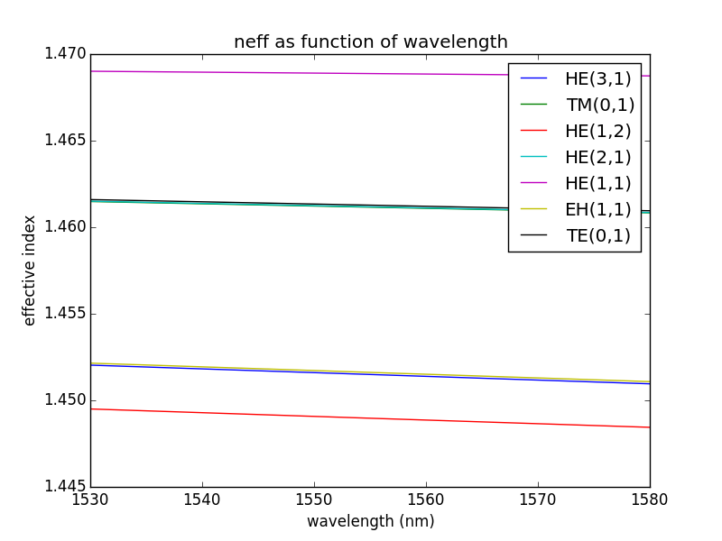
Plotting neff as function of the wavelength¶

In this second example, we will plot neff as function of the wavelength, for a single fiber. First, we import the modules we need, we define the list of wavelengths we want to simulate, as well as the FiberFactory we will use:

import numpy
from matplotlib import pyplot
from fibermodes import FiberFactory, Simulator

wavelengths = numpy.linspace(1530e-9, 1580e-9, 11)
factory = FiberFactory()
factory.addLayer(radius=4e-6, index=1.474)
factory.addLayer()

Then we build the Simulator object, and we compute the effective indexes:

sim = Simulator(factory, wavelengths, delta=1e-5)
neffiter = sim.neff()

The delta parameter, passed to the Simulator constructor, is simply the interval used by the solver to find the characteristic function zeros. An higher value decrease computation time, but increase the risk to skip some zeros. A lower value increase computation time, but increase the risk to skip some roots. Usually, an highly multimode fiber will require a lower delta. The neff() function returns an iterator. In the current example, it yields only one value, because the FiberFactory produces a single fiber. If the FiberFactory was defining many fibers, the returned iterator would yield values for each generated fiber. Since we only have one value to consume, we can simply call next() on it:

neffs = next(neffiter)

The value returned by the iterator is a list. Each item of the list correspond to one wavelength. Since our simulator has 11 wavelengths, neffs is a list of 11 items. Each item of the list is a dictionary. The keys of the dictionary are the different supported modes, for that combination of fiber and wavelength. We now need to transform this structure to an array, suitable for matplotlib. Because we want one line per mode, we first iterate over the list of modes. The number of supported modes can vary with the wavelength; however, the smallest wavelength should support the highest number of modes. This is why we can use the list of modes from the first wavelength:

for mode in next(sim.modes())[0]:
    neff = []
    for neffwl in neffs:  # for each wavelength
        try:
            neff.append(neffwl[mode])
        except KeyError:  # mode not supported
            neff.append(float("nan"))
    neffma = numpy.ma.masked_invalid(neff)  # mask "nan"
    pyplot.plot(wavelengths, neffma, label=str(mode))
pyplot.legend()
pyplot.show()

Simulator accepts most functions of Fiber, including neff(), b(), vp(), ng(), vg(), D(), and S(). It also have the modes() function, that returns the list of supported modes. Finally, it has beta0(), beta1(), beta2() and beta3() functions to get the beta parameter and its derivatives.

Using Simulator¶

Counting modes and finding cutoffs¶

Plotting neff as function of the wavelength¶

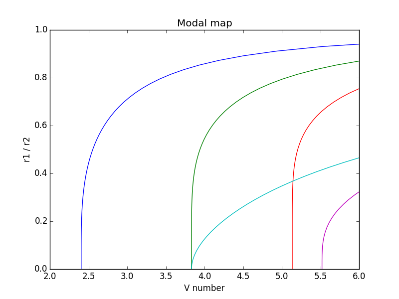
Plotting modal map¶